Workshop Slides

Author

Affiliation

Dr Taren Sanders

Institute for Postive Psychology and Education, Australian Catholic University

Published

21 April 2023

Before We Start

Please go to

bit.ly/GGIRWorkshop

and follow the Getting Started instructions.

Introduction

Why Me?

More than a decade working with accelerometers
Projects with >25k accelerometers
Contributed code to GGIR
Developed packages for distributed processing

Overview of the workshop

Objectives

Understand why open-source methods matter
Have a basic understanding of R
Understand how to process accelerometer data with GGIR, and interpret the output

Agenda

The advantages (and some disadvantages) of using open-source processing methods
The basics of using R
Installing and running GGIR
Understanding the settings and options
Interpreting the output
Common issues and troubleshooting steps
Advanced options (e.g., day segment analysis)

Understanding Accelerometer Data and the Need for GGIR

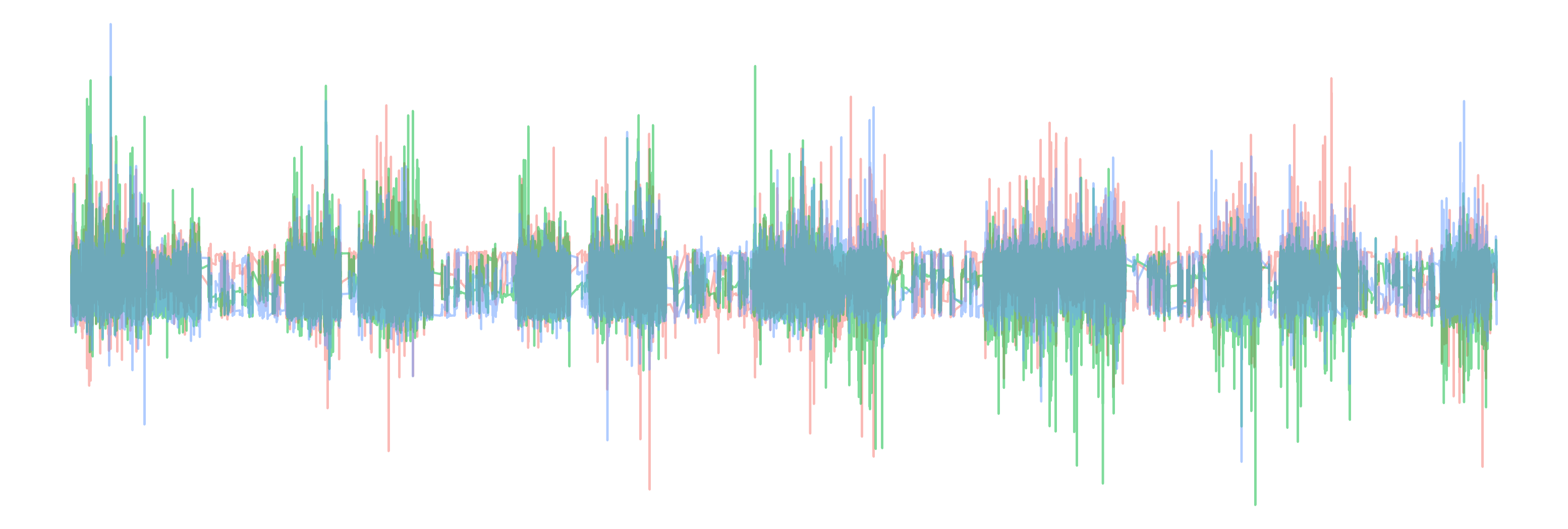
Basics of accelerometer data

Limitations of proprietary methods

Limited transparency
Limited scalability
Limited extensability
Vendor lock-in

Why GGIR?

Multi-device
New and expanding features
Open-source nature
Scalable and extensible

What do we really want to know?

How much? (Volume)
How hard? (Intensity)

Physical activity metrics

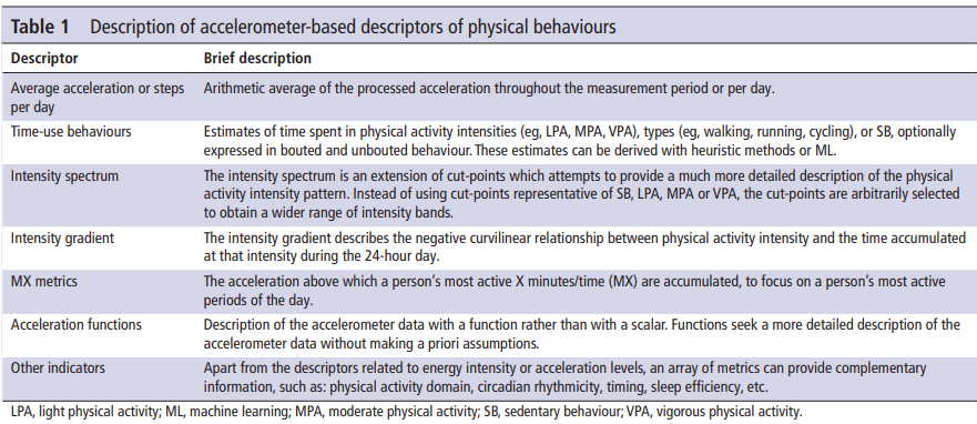
New(er) physical activity metrics

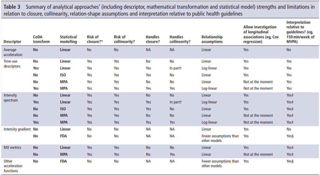
MX Metrics

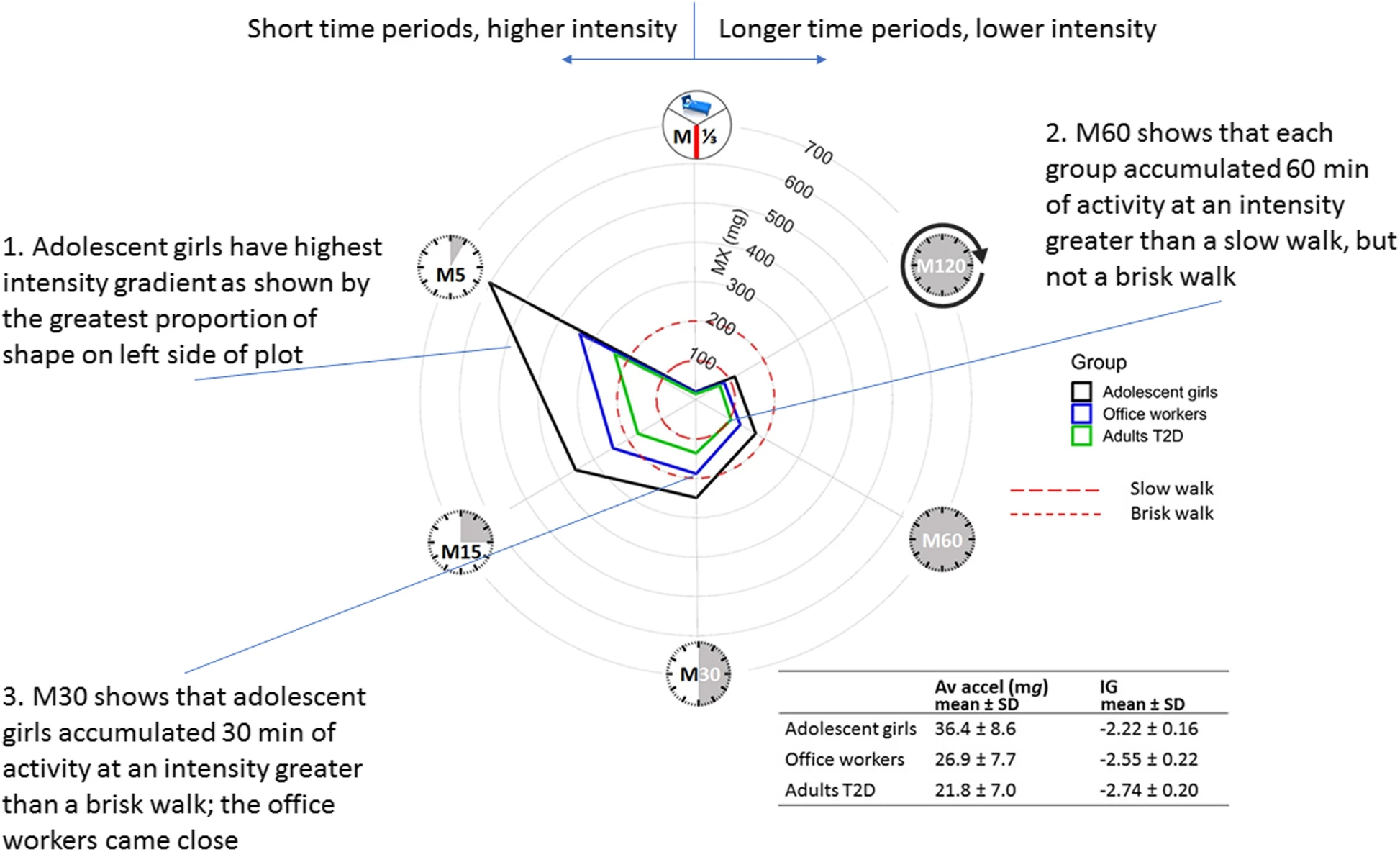
Remember that we are measuring accelerations, and translating these to physical activity. By focusing on the actual accelerations, we avoid the translation errors.

New(er) physical activity metrics

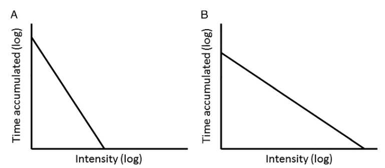
Intensity Gradient

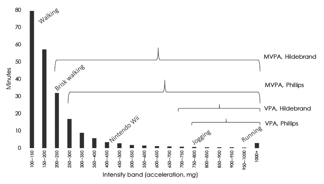
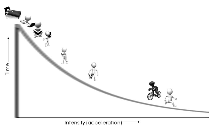
New(er) physical activity metrics

Intensity Gradient

Why GGIR?

Calculate all of these metrics at once

A (Very) Quick Intro to R

What is R?

R is a free, open-source programming language
Specially designed for data analysis and statistics
Widely used in research, data science, and industry

An example

Fitting a simple linear model:

\[\hat{y} = \beta_0 + \beta_1x\]

. . .

R Code

# Fit a linear model
lm(y ~ x)

. . .

Python Code

# Import packages
import numpy as np
import statsmodels.api as sm

# Add a constant term to x (statsmodels doesn't add one by default)
x = sm.add_constant(x)

# Fit the linear model
model = sm.OLS(y, x).fit()

Why use R?

Pros

Free
Reproducible
Extensive set of add-on tools and packages
Typeset as you go

Cons

Steeper learning curve than point-and-click interfaces

R Resources

R for Data Science

r4ds.had.co.nz

Software Carpentry

swcarpentry.github.io

Activity: Intro to R

Processing Accelerometer Data with GGIR

Understanding what GGIR is doing

Understanding what GGIR is doing

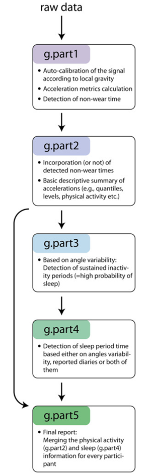
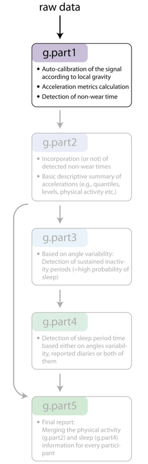
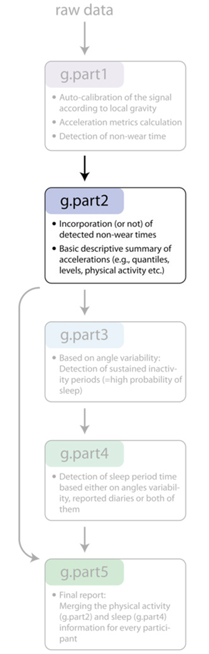
Part 1

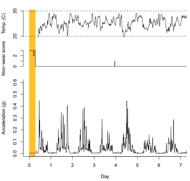
Pre-processing steps
Acceleration metrics (data collapsed)
Non-wear detection and imputation
Longest time to complete

Understanding what GGIR is doing

Part 2

Data imputation
Physical activity calculation
Output: Part 2 reports, data quality plots

Understanding what GGIR is doing

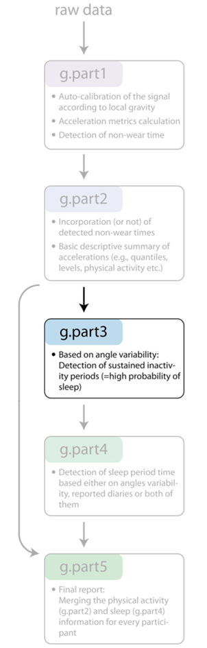
Part 3

Detection of sustained inactivity
Estimate start/end period of sleep window

Understanding what GGIR is doing

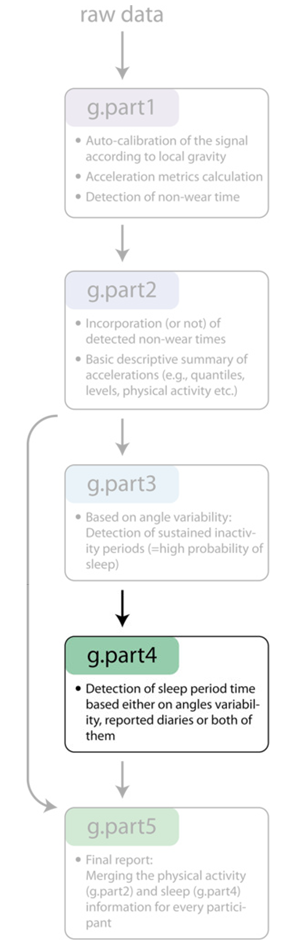
Part 4

Convert detected inactivity in sleep window to sleep
Or use sleep diary for sleep window
Output: Part 4 reports

Understanding what GGIR is doing

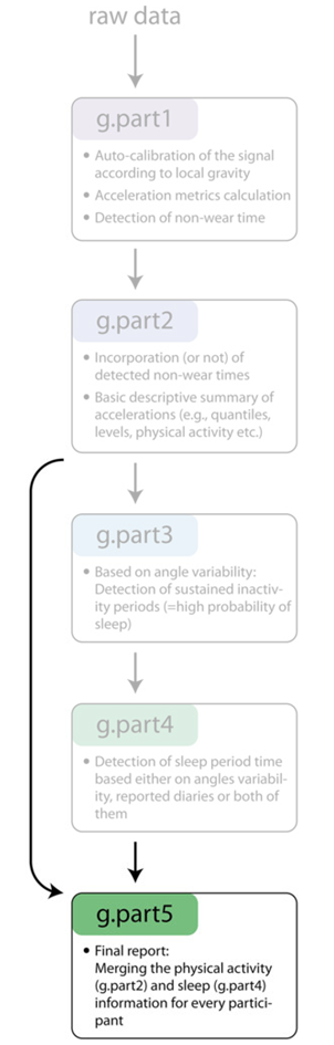
Part 5

Collate data from Part 2 and Part 4 for final report
Output: Part 5 reports

Running the main GGIR function

All options

GGIR(
  mode,
  datadir,
  f0,
  f1,
  windowsizes,
  desiredtz,
  overwrite,
  do.parallel,
  maxNcores,
  myfun,
  outputdir,
  studyname,
  chunksize,
  do.enmo,
  do.lfenmo,
  do.en,
  do.bfen,
  do.hfen,
  do.hfenplus,
  do.mad,
  do.anglex,
  do.angley,
  do.angle,
  do.enmoa,
  do.roll_med_acc_x,
  do.roll_med_acc_y,
  do.roll_med_acc_z,
  do.dev_roll_med_acc_x,
  do.dev_roll_med_acc_y,
  do.dev_roll_med_acc_z,
  do.lfen,
  do.lfx,
  do.lfy,
  do.lfz,
  do.hfx,
  do.hfy,
  do.hfz,
  do.bfx,
  do.bfy,
  do.bfz,
  do.zcx,
  do.zcy,
  do.zcz,
  lb,
  hb,
  n,
  do.cal,
  spherecrit,
  minloadcrit,
  printsummary,
  print.filename,
  backup.cal.coef,
  rmc.noise,
  rmc.dec,
  rmc.firstrow.acc,
  rmc.firstrow.header,
  rmc.col.acc,
  rmc.col.temp,
  rmc.col.time,
  rmc.unit.acc,
  rmc.unit.temp,
  rmc.origin,
  rmc.header.length,
  mc.format.time,
  rmc.bitrate,
  rmc.dynamic_range,
  rmc.unsignedbit,
  rmc.desiredtz,
  rmc.sf,
  rmc.headername.sf,
  rmc.headername.sn,
  rmc.headername.recordingid,
  rmc.header.structure,
  rmc.check4timegaps,
  rmc.col.wear,
  rmc.doresample,
  imputeTimegaps,
  selectdaysfile,
  dayborder,
  dynrange,
  configtz,
  minimumFileSizeMB,
  interpolationType,
  expand_tail_max_hours,
  metadatadir,
  minimum_MM_length.part5,
  strategy,
  hrs.del.start,
  hrs.del.end,
  maxdur,
  max_calendar_days,
  includedaycrit,
  L5M5window,
  M5L5res,
  winhr,
  qwindow,
  qlevels,
  ilevels,
  mvpathreshold,
  boutcriter,
  ndayswindow,
  idloc,
  do.imp,
  storefolderstructure,
  epochvalues2csv,
  do.part2.pdf,
  mvpadur,
  window.summary.size,
  bout.metric,
  closedbout,
  IVIS_windowsize_minutes,
  IVIS_epochsize_seconds,
  IVIS.activity.metric,
  iglevels,
  TimeSegments2ZeroFile,
  qM5L5,
  MX.ig.min.dur,
  qwindow_dateformat,
  anglethreshold,
  timethreshold,
  acc.metric,
  ignorenonwear,
  constrain2range,
  do.part3.pdf,
  sensor.location,
  HASPT.algo,
  HASIB.algo,
  Sadeh_axis,
  longitudinal_axis,
  HASPT.ignore.invalid,
  loglocation,
  colid,
  coln1,
  nnights,
  sleeplogidnum,
  do.visual,
  outliers.only,
  excludefirstlast,
  criterror,
  includenightcrit,
  relyonguider,
  relyonsleeplog,
  def.noc.sleep,
  data_cleaning_file,
  excludefirst.part4,
  excludelast.part4,
  sleeplogsep,
  sleepwindowType,
  excludefirstlast.part5,
  boutcriter.mvpa,
  boutcriter.in,
  boutcriter.lig,
  threshold.lig,
  threshold.mod,
  threshold.vig,
  timewindow,
  boutdur.mvpa,
  boutdur.in,
  boutdur.lig,
  save_ms5rawlevels,
  part5_agg2_60seconds,
  save_ms5raw_format,
  save_ms5raw_without_invalid,
  includedaycrit.part5,
  frag.metrics,
  LUXthresholds,
  LUX_cal_constant,
  LUX_cal_exponent,
  LUX_day_segments,
  do.sibreport
)

Running the main GGIR function

Minimum options

GGIR(
  datadir,
  outputdir
)

Running the main GGIR function

Good starting place

GGIR(
  mode = c(1, 2, 3, 4, 5),
  datadir = "C:/mystudy/mydata",
  outputdir = "D:/myresults",
  # =====================
  # Part 2
  # =====================
  idloc = 2,
  strategy = 2,
  maxdur = 9,
  includedaycrit = 16,
  qwindow = c(0, 24),
  qlevels = c(
    960 / 1440,   # Top 8 hours
    1320 / 1440,  # Top 120min
    1380 / 1440,  # Top 60min
    1410 / 1440,  # Top 30min
    1425 / 1440,  # Top 15min
    1435 / 1440), # Top 5min
  ilevels = seq(0, 4000, 50),
  iglevels = 1,
  mvpathreshold = c(100),
  mvpadur = c(1, 5, 10),
  boutcriter = 0.8,
  # =====================
  # Part 3 + 4
  # =====================
  def.noc.sleep = 1,
  excludefirstlast = FALSE,
  includenightcrit = 16,
  # =====================
  # Part 5
  # =====================
  threshold.lig = c(30), threshold.mod = c(100), threshold.vig = c(400),
  boutcriter.in = 0.9, boutcriter.lig = 0.8, boutcriter.mvpa = 0.8,
  boutdur.in = c(1, 10, 30), boutdur.lig = c(1, 10), boutdur.mvpa = c(1),
  includedaycrit.part5 = 16,
  timewindow = c("MM", "WW"),
  # =====================
  # Reports
  # =====================
  visualreport = TRUE,
  do.report = c(2, 4, 5)
)

idloc = how to extract the ID number

strategy = how study was setup. 2 means use data between first and last midnight. You can also use strategies based on cutting off hours at the start or end, the most active days, or just everything after the first midnight.

maxdur = max number of days accel was worn. Useful if you know you’ll have a lot of non-wear time at the end.

qwindow = Periods to calculate the variables over. Useful for day segement analysis (we’ll come back to this).

qlevels = method to calculate the MX metrics

ilevels = calculate the amount of time in each of these ‘bins’. These would produce the same graph as we saw in the intensity gradients

iglevels = if you provide a number, it will calculate the intensity gradient. Can also set your own bins here, but the defaults are fine.

mvpadur = bout durations for MVPA (in minutes)

boutcriter = proportion of bout that needs to be above threshold

def.noc.sleep = how to define the sleep window. You can provide a time period, or use the least active 12 hours. Using a single number will use a detection algorithm.

includenightcrit = number of hours (between noon and noon) that need to be valid for sleep to be calculated

timewindow = period over which statistics are calculated. Either midnight to midnight (always = 1440) or wake to wake.

visualreport = combined report of part 2 and 4. Useful for particpants.

do.report = which sections to produce csv files from.

Activity: Basic GGIR Processing

Interpreting the Output

Output contents

meta/
- Milestone data
- Sleep data quality plots
results/
- Reports from each part
- QC/
  - Uncleaned versions of reports
- file summary reports/
  - Summary reports for participants
config.csv

Report contents

‘summary’ vs ‘day|night|person summary’
If you’ve done part 5, the results you want are probably there

GGIR column names

Column names from GGIR can be hard to follow!
The vignette is a great resource.

Understanding the output files

Part 5

Some of the key abbreviations:

Averages: _pla (plain); _wei (weighted); _WD (weekday); _WE (weekend)
Intensities: IN (inactive); LIG (light); MOD (moderate); VIG (vigorous)

Some of the key columns:

Nvaliddays*
dur_day_total_[IN|LIG|MOD|VIG]_min
ACC_day_mg
ig_gradient
dur_spt_min
sleep_efficiency

Understanding the output files

Part 4

Some of the key columns (not in part 5):

SleepRegularityIndex

Understanding the output files

Part 2

Some of the key abbreviations:

Averages: AD (all days); WD (weekday); WE (weekend); WWD (weighted weekday); WWE (weighted weekend)

Some of the key columns (not in part 5):

AD_p99.65278_ENMO_mg_0.24hr (MX metrics)
AD_.0.50._ENMO_mg_0.24hr (ilevels)

Activity: Code breaking

Find a column in one of the outputs that is confusing, and see if you can decipher it using the vignette

Exploring Other Options in GGIR

Running in Multiple Steps

Part 1 can be run first (e.g., left overnight), before experimenting with parts 2-5.
If you make changes to parts 2-5, remember to set overwrite = TRUE.

# Run Part 1
GGIR(
  mode = 1,
  datadir = "C:/mystudy/mydata",
  outputdir = "C:/myresults",
  # Any other Part 1 args
)

# Run Parts 2-5
GGIR(
  mode = c(2, 3, 4, 5),
  datadir = "C:/mystudy/mydata",
  outputdir = "C:/myresults",
  overwrite = TRUE
  # Your part 2-5 arguments
)

Day Segmentation

Clock based

Great for when all particpants share the same schedule you want to test.
Just provide additional values in qwindow
Note that this complicates qlevels

Example: You want to see if your intervention improves physical activity during school, or if there are changes before or after school. School runs from 8:30am to 3:15pm.

GGIR(
  mode = c(1, 2, 3, 4, 5),
  datadir = "C:/mystudy/mydata",
  outputdir = "D:/myresults",
  ... # Other args
  qwindow = c(0, 8.5, 15.25, 24),
  ... # Other args
)

Day Segmentation

Activity log based

Used when participants have varied schedules
You will need a participant-completed activity log, formatted correctly
Provide this log to qwindow
qlevels is almost impossible for anything other than overall

Example: You are interested in physical activity during people’s commutes. Participants completed a daily log of when they commuted.

id	date	to_work	work	from_work	home	date	to_work	work	from_work	home
201	26-05-2017	08:15:00	08:30:00	17:00:00	17:31:00	27-05-2017				17:31:00
202	25-05-2017	07:25:00	08:00:00	16:50:00	17:20:00	26-05-2017	07:25:00	08:00:00	16:50:00	17:20:00
203	27-05-2017	08:11:00	09:01:00	17:11:00	17:55:00	28-05-2017	08:11:00	09:01:00	17:11:00	17:55:00

GGIR(
  mode = c(1, 2, 3, 4, 5),
  datadir = "C:/mystudy/mydata",
  outputdir = "D:/myresults",
  ... # Other args
  qwindow = "C:/mystudy/myactivitylogs.csv",
  ... # Other args
)

Using different cut-points

There’s a great write up of published cut-points and how to use them
In some cases, you need to use a different Part 1 metric (e.g., ENMOa)

Activity: Challenges

Q&A

Contact Details

Dr Taren Sanders

Institute for Positive Psychology and Education, Australian Catholic University

Taren.Sanders@acu.edu.au